Logistic regression: Difference between revisions
No edit summary |
No edit summary |
||
| (3 intermediate revisions by the same user not shown) | |||
| Line 1: | Line 1: | ||
[[Category:Machine Learning]] | |||
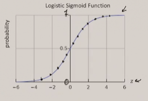
[[File:Logistic regression sigmoid.png|thumb|Figure 1. The shape of the logistic regression function is an S]] | [[File:Logistic regression sigmoid.png|thumb|Figure 1. The shape of the logistic regression function is an S]] | ||
'''Logistic regression''' uses the logistic function (sigmoid) to map the output of a linear regression function <math>z</math> to 0 or 1. | '''Logistic regression''' uses the logistic function (sigmoid) to map the output of a linear regression function <math>z</math> to 0 or 1. | ||
| Line 11: | Line 12: | ||
As shown in figure 1, the sigmoid is S-shaped. It is a good approximation of the transition from 0 to 1. | As shown in figure 1, the sigmoid is S-shaped. It is a good approximation of the transition from 0 to 1. | ||
As stated in the last section, we feed the output of linear regression into sigmoid. | As stated in the last section, we feed the output of linear regression into sigmoid. Sigmoid outputs a probability of 1. | ||
<math> | <math> | ||
sigm(z=wx)=\frac{1}{1+e^{-z}} | sigm(z=wx)=\frac{1}{1+e^{-z}} | ||
</math> | </math> | ||
= Decision boundary = | |||
The '''decision boundary''' is the threshold above which the input can be classified as 1. After the logistic function gives the probability of the event, a decision boundary can be set depending on the scenario. | |||
In normal cases, the decision boundary is set to 0.5. Sometimes, you want to be more than 50% sure before classifying an output to 1. This means shifts to the decision boundary. | |||
= Loss function = | |||
Based on the principle of [[Maximum likelihood estimation|MLE]], the loss function is the probability of seeing the data given our model. | |||
<math> | |||
L(w|X)=\prod g(x^{(i)},w)^{y^{(i)}}\left( 1 - g(x^{(i)},w) \right)^{1 - y^{(i)}} | |||
</math> | |||
The probability is based on Bernoulli distribution. Same as in MLE, we use log to reduce computational complexity. I'm too lazy to type it out. | |||
Latest revision as of 19:34, 17 May 2024

Logistic regression uses the logistic function (sigmoid) to map the output of a linear regression function to 0 or 1.
Linear regression
Linear regression cannot be directly used for (binary) classification. Indirectly, a threshold is used. When the value is above the threshold, it is considered 1; when it is below, it is considered 0.
Classification using linear regression is sensitive to the threshold. The problem with this approach is the difficulty in determining a good threshold. Logistic regression mitigates that by feeding into a logistic function.
Logistic function
As shown in figure 1, the sigmoid is S-shaped. It is a good approximation of the transition from 0 to 1.
As stated in the last section, we feed the output of linear regression into sigmoid. Sigmoid outputs a probability of 1.
Decision boundary
The decision boundary is the threshold above which the input can be classified as 1. After the logistic function gives the probability of the event, a decision boundary can be set depending on the scenario.
In normal cases, the decision boundary is set to 0.5. Sometimes, you want to be more than 50% sure before classifying an output to 1. This means shifts to the decision boundary.
Loss function
Based on the principle of MLE, the loss function is the probability of seeing the data given our model.
The probability is based on Bernoulli distribution. Same as in MLE, we use log to reduce computational complexity. I'm too lazy to type it out.


