Sampling Distribution

Let there be Failed to parse (SVG (MathML can be enabled via browser plugin): Invalid response ("Math extension cannot connect to Restbase.") from server "https://wikimedia.org/api/rest_v1/":): {\displaystyle Y_1, Y_2, \ldots, Y_n } , where each Failed to parse (SVG (MathML can be enabled via browser plugin): Invalid response ("Math extension cannot connect to Restbase.") from server "https://wikimedia.org/api/rest_v1/":): {\displaystyle Y_i} is a randomv variable from the population.

Every Y have the same mean and distribution that we don't know.

Failed to parse (SVG (MathML can be enabled via browser plugin): Invalid response ("Math extension cannot connect to Restbase.") from server "https://wikimedia.org/api/rest_v1/":): {\displaystyle E(Y_i) = \mu, Var(Y_i) = \sigma^2 }

We then have the sample mean

Failed to parse (SVG (MathML can be enabled via browser plugin): Invalid response ("Math extension cannot connect to Restbase.") from server "https://wikimedia.org/api/rest_v1/":): {\displaystyle \bar{Y} = \frac{1}{n} \sum_{i = 1}^n Y_i }

The sample mean is expected to be Failed to parse (SVG (MathML can be enabled via browser plugin): Invalid response ("Math extension cannot connect to Restbase.") from server "https://wikimedia.org/api/rest_v1/":): {\displaystyle \mu} through a pretty easy direct proof

The variance of the sample mean is Failed to parse (SVG (MathML can be enabled via browser plugin): Invalid response ("Math extension cannot connect to Restbase.") from server "https://wikimedia.org/api/rest_v1/":): {\displaystyle \frac{\sigma^2}{n}} , also through a pretty easy direct proof.

Central limit theorem

The central limit theorem states that the distribution of the sample mean follows normal distribution.

Failed to parse (SVG (MathML can be enabled via browser plugin): Invalid response ("Math extension cannot connect to Restbase.") from server "https://wikimedia.org/api/rest_v1/":): {\displaystyle \bar{Y} \sim N(\mu, \frac{\sigma^2}{n})}

As long as the following two conditions are satisfied, CLT applies, regardless of the population's distribution.

1. The population distribution of Failed to parse (SVG (MathML can be enabled via browser plugin): Invalid response ("Math extension cannot connect to Restbase.") from server "https://wikimedia.org/api/rest_v1/":): {\displaystyle Y} is normal, or
2. The sample size for each $Y_{i}$ is large $n>30$

By extension, we also have the distribution of the sum.

$S\sim N(\mu _{S}=n\mu ,\sigma _{S}={\sqrt {n\sigma }})$

where $S=\sum Y_{i}$

Proportion Approximation

The sampling distribution of the proportion of success of n bernoulli random variables (${\hat {p}}$) can also be approximated to a normal distribution under the CLT.

Consider bernoulli random variables

$Y_{1}\ldots Y_{n}\sim E(Y_{i})=p,Var(Y_{i})=p(1-p)$

The proportion of success ${\hat {p}}$ is the sum over the count, so the expected probability is

$E({\hat {p}})=E\left({\frac {1}{n}}\sum Y_{i}\right)=p$

and the variance of ${\hat {p}}$ is

$Var\left({\frac {1}{n}}\sum Y_{i}\right)={\frac {1}{n^{2}}}Var\left(\sum Y_{i}\right)={\frac {p(1-p)}{n}}$

With a large sample size n, we can appoximate this to a normal distribution. Notably, the criteria for a large n is different from that of the continuous random variable.

$np>5,n(1-p)>5$

then we have

${\hat {p}}\sim N\left(p,{\frac {p(1-p)}{n}}\right)$

The reasoning behind the weird criteria relates to the binomial distribution. It's not very elaborated on in the lecture, but $np$ is the mean of the binomial (i.e. the expected number of successes). The criteria essentially makes sure that no negative values are plausible in the approximation; with a small mean and a large variance, the left side of a normal approximation goes into the negative, but bernoulli/binomial must always be positive.

Binomial Approximation

I'm short on time. This is based on the above section and a bit of math.

$Y\sim N(np,np(1-p))$

Confidence Interval

Estimation is the guess for the unknown parameter. A point estimate is a "best guess" of the population parameter, where as the confidence interval is the range of reasonable values that are intended to contain the parameter of interest with a certain degree of confidence, calculated with

(point estimate - margin of error, point estimate + margin of error)

Standard Error

The standard error measures how much error we expect to make when estimating $\mu _{Y}$ by ${\bar {y}}$.

Constructing CIs

By CLT, ${\bar {Y}}\sim N(\mu ,{\frac {\sigma ^{2}}{n}})$. The confidence interval is the range of plausible ${\bar {Y}}$.

If we define the middle 90% to be plausible, to find the confidence interval, simply find the 5th and 95th percentile.

Generalized, if we want a confidence interval of the middle Failed to parse (SVG (MathML can be enabled via browser plugin): Invalid response ("Math extension cannot connect to Restbase.") from server "https://wikimedia.org/api/rest_v1/":): {\displaystyle (1 - \alpha) 100%} , have a confidence interval of

Failed to parse (SVG (MathML can be enabled via browser plugin): Invalid response ("Math extension cannot connect to Restbase.") from server "https://wikimedia.org/api/rest_v1/":): {\displaystyle \bar{y} \pm Z_{\alpha / 2} \frac{\sigma}{ \sqrt{n} } }

where Failed to parse (SVG (MathML can be enabled via browser plugin): Invalid response ("Math extension cannot connect to Restbase.") from server "https://wikimedia.org/api/rest_v1/":): {\displaystyle \bar{y}} is the sample mean and Failed to parse (SVG (MathML can be enabled via browser plugin): Invalid response ("Math extension cannot connect to Restbase.") from server "https://wikimedia.org/api/rest_v1/":): {\displaystyle Z_{x}} is the z score of the x-th percentile.

T-Distribution

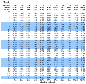
T distribution table

CLT is based on the population variance. Since we don't know the population variance Failed to parse (SVG (MathML can be enabled via browser plugin): Invalid response ("Math extension cannot connect to Restbase.") from server "https://wikimedia.org/api/rest_v1/":): {\displaystyle \sigma^2} , we have to use the sample variance Failed to parse (SVG (MathML can be enabled via browser plugin): Invalid response ("Math extension cannot connect to Restbase.") from server "https://wikimedia.org/api/rest_v1/":): {\displaystyle s} to estimate it. This introduces more uncertainty, accounted for by the t-distribution.

T-distribution is the distribution of sample mean based on population mean, sample variance and degrees of freedom (covered later). It looks very similar to normal distribution.

When the sample size Failed to parse (SVG (MathML can be enabled via browser plugin): Invalid response ("Math extension cannot connect to Restbase.") from server "https://wikimedia.org/api/rest_v1/":): {\displaystyle n} is small, there is greater uncertainty in the estimates. T-di

Failed to parse (SVG (MathML can be enabled via browser plugin): Invalid response ("Math extension cannot connect to Restbase.") from server "https://wikimedia.org/api/rest_v1/":): {\displaystyle t_{\alpha/2} > Z_{\alpha/2} }

The spread of t-distribution depends on the degrees of freedom, which is based on sample size. When looking up the table, round down df.

Failed to parse (SVG (MathML can be enabled via browser plugin): Invalid response ("Math extension cannot connect to Restbase.") from server "https://wikimedia.org/api/rest_v1/":): {\displaystyle \upsilon = n - 1 }

As the sample size increases, degrees of freedom increase, the spread of t-distribution decreases, and t-distribution approaches normal distribution.

Based on CLT and normal distribution, we had the confidence interval

Failed to parse (SVG (MathML can be enabled via browser plugin): Invalid response ("Math extension cannot connect to Restbase.") from server "https://wikimedia.org/api/rest_v1/":): {\displaystyle \bar{Y} \pm Z_{\alpha / 2} \frac{\sigma}{ \sqrt{n} } }

Now, based on T-distribution, we have the CI

Failed to parse (SVG (MathML can be enabled via browser plugin): Invalid response ("Math extension cannot connect to Restbase.") from server "https://wikimedia.org/api/rest_v1/":): {\displaystyle \bar{Y} \pm t_{\alpha / 2} \frac{s}{ \sqrt{n} } }

Find Sample Size

To calculate sample size needed depending on desired error margin and sample variance by assuming that Failed to parse (SVG (MathML can be enabled via browser plugin): Invalid response ("Math extension cannot connect to Restbase.") from server "https://wikimedia.org/api/rest_v1/":): {\displaystyle \upsilon = \infty}

Failed to parse (SVG (MathML can be enabled via browser plugin): Invalid response ("Math extension cannot connect to Restbase.") from server "https://wikimedia.org/api/rest_v1/":): {\displaystyle n = \frac{Z^2_{\alpha/2} s^2}{E^2} }

We want to always round up to stay within the error margin.

I don't really know why.

Sampling Distribution of Difference

By linear combination of RVs, sampling distribution of Failed to parse (SVG (MathML can be enabled via browser plugin): Invalid response ("Math extension cannot connect to Restbase.") from server "https://wikimedia.org/api/rest_v1/":): {\displaystyle \bar{Y_1} - \bar{Y_2}} is

Failed to parse (SVG (MathML can be enabled via browser plugin): Invalid response ("Math extension cannot connect to Restbase.") from server "https://wikimedia.org/api/rest_v1/":): {\displaystyle ( \bar{Y_1} - \bar{Y_2} ) \sim N(\mu_1 - \mu_2, \frac{\sigma_1^2}{n_1} + \frac{\sigma_2^2}{n_2}) }

However, we do not know the population variance Failed to parse (SVG (MathML can be enabled via browser plugin): Invalid response ("Math extension cannot connect to Restbase.") from server "https://wikimedia.org/api/rest_v1/":): {\displaystyle \sigma^2} . If the CLT assumptions hold, then we have

Failed to parse (SVG (MathML can be enabled via browser plugin): Invalid response ("Math extension cannot connect to Restbase.") from server "https://wikimedia.org/api/rest_v1/":): {\displaystyle \upsilon = \frac{ \left( \frac{s_1^2}{n_1} + \frac{s_2^2}{n_2} \right)^2 }{ \frac{(s_1^2 / n_1)^2 }{n_1 - 1} + \frac{(s_2^2 / n_2)^2 }{n_2 - 1} } }

Trust me bro. Remember to round down to use t-table. With this degree of freedom, we can use sample variance to estimate the distribution.